Since the inception of spreadsheet applications for the PC desktop computer, tabular reports are easy and quick to create including dynamic calculations (calculation performed in real-time).
In my opinion, spreadsheets serve as the best “calculators” alternative when several data items and computations are a necessity.
A spreadsheet cannot only perform simple dynamic calculator-type functions, but can incorporate formatting of cells such as color, highlighting, underlining, etc.
This process was originally documented in late 2010 and posted years later… 🙁
This post focuses on a very simple spreadsheet application using Microsoft (MS) Excel by creating a student grade roster as illustrated below.
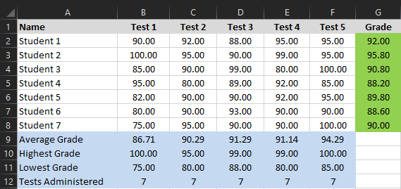
Calculating Student Test Scores using MS Excel
The following is hypothetical and meant to be serve as an educational and learning experience.
Problem Statement:
As an educational professional, you want to create a spreadsheet reusable for the various class sections you teach in your educational institution. Simply, the spreadsheet will store student name, grades for given exams to determine a final grade. In addition, for each test (exam), exhibit average, highest, and lowest grade as shown in the final product figure above.
Let’s get started!!
1) Seed student data
Open MS Excel with a blank spreadsheet.
Enter the below data into each cell (A1 to F8) including headings.
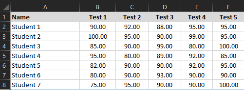
Optionally, you may format column headings as bold with grey background. (e.g. Name)
2) Add student final grade
In cell G1, add new column heading (Grade) to represent students final grade.
Cell G2 declares a formula which calculates Student 1 final grade by computing the average of 5 test scores administered during the term.
The formula content in cell G2 could be “=(b2+c2+d2+e2+f2)/5”. However, a more flexible formula is “=SUM(B2:F2)/(COUNT(B2:F2))” which states:
SUMmarize cells B2 through F2 and divide by COUNT of B2 through F2 giving a final grade of 92.00!

Propagate the formula from cell G2 to other student cells, G3 to G8, as depicted in the automated GIF below (figure-4).
Select cell G2 and position cursor on the lower right corner until the cursor changes to a plus (+) sign.
Click and hold the right mouse button dragging downwards to cell G8. Note, the cell border is extending downwards as shown below. Release mouse hold when cell G8 is reached. The formula will be copied to each cell and final grade calculation will occur “like magic” for each of the remaining students!!
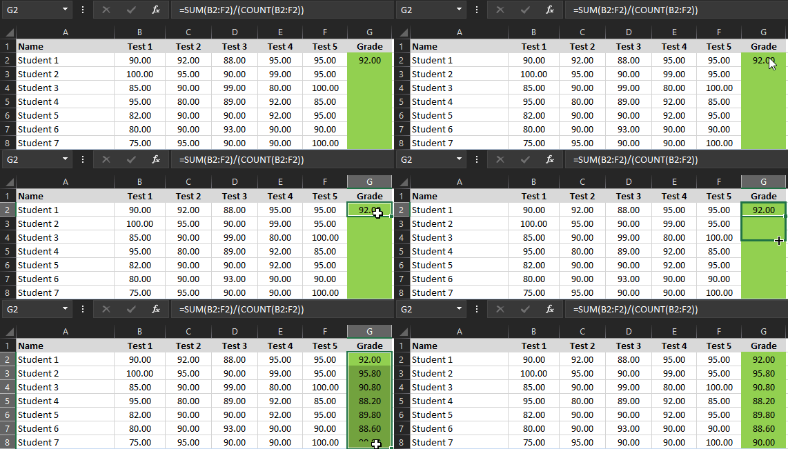
Figure-4: Propagate grade formula to remaining students
3) Add average grade
In cell A9, type “Average Grade” as heading.
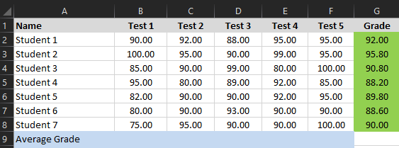
Cell B9 declares a formula which calculates the average grade for Test 1 by calculating the average of the 5 individual test scores administered during the term.
The formula content in cell B9 is “=(b2+b3+b4+b5+b6+b7+b8)/7”. However, a more flexible formula using the SUM and COUNT functions is “=SUM(B2:B8)/(COUNT(B2:B8))” which states:
SUMmarize cells B2 through B8 and divide by COUNT of B2 through B8 giving a average test grade of 86.71!
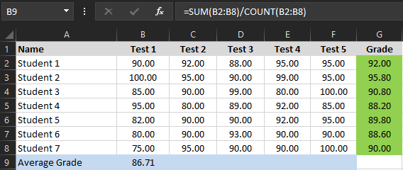
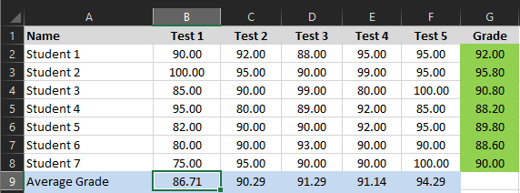
Propagate the average grade formula from cell B1 to cells C9 through F9 using the procedure from step 2 (position on cell B9, place cursor on lower right corner until cursor changes to a plus sign, hold-n-drag to cell F9, and release hold).
Figure 7 exhibits results after propagation.
4) Add highest grade, lowest grade and tests administered
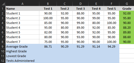
Add three rows (refer to figure 8):
- In cell A10 type “Highest Grade” as heading
- In cell A11 type “Lowest Grade” as heading
- In cell A12 type “Tests Administered” as heading
Add three formula sets (refer to figure 9):
- Add formula in cell B10 using the MAXimum function, “=MAX(B2:B8)” which states:
display MAXimum value from cells B2 through B8 yielding 100 - Add formula in cell B11 using the MINimum function, “=MIN(B2:B8)” which states:
display MAXimum value from cells B2 through B8 yielding 75 - Add formula in cell B12 using the COUNT function, “=COUNT(B2:B8)” which states:
count values from cells B2 through B8 yielding 7
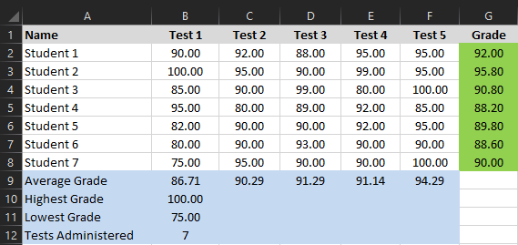
Propagate each new formula (e.g. cell B10) using the procedure from step 2 (final grade) but drag-n-hold to the right until reaching cell containing last test (e.g. cell F10).
Figure 10 exhibits results after propagation.

5) Done
Congratulations! You can now apply or modify the test grade roster per your needs.
Enjoy,
Larry Belmontes
Download
The MS Excel (version 2016) spreadsheet created in this post can be downloaded from here as a zip file.